Graham explains the key points in the latest round of TAG updates. Another bumper edition, extending into 2025

Updated (23 November 2024) to reflect publication of the supplementary guidance for the “new mode problem” and the OBR’s October 2024 medoum-term forecasts.

The DfT has published some details of the latest round of updates to its Transport Analysis Guidance (TAG). There are three Forthcoming Change (FC) notices, covering different aspects, but (as with the last couple of rounds) we mostly don’t yet have the full text of the updated units or an updated Databook. I’d expect these to come through in November when most updates are due to go live, and I will update this post when they do. For now, we just have what’s in the FC notices.

The changes include:

• Routine updates to the economic and demographic data, including a significant update to the population projection
• Minor updates to the emissions factors
• A correction to the landscape monetisation workbook
• Some intriguing extra guidance on optimism bias for rail opex
• A slate of technical changes to wider economic impacts
• An honorary mention for an extra version of the BCR
• And a new method for the “new mode problem”.

I’ll shortly update my Tag-at-a-Glance page to give a unit-by-unit summary of these changes. This post just covers the highlights and some of the background to them.

Updated economic and demographic data

The economic and population forecasts in the TAG Databook are routinely updated with the latest data from the Office for National Statistics (ONS) and the Office for Budget Responsibility (OBR).

This autumn’s updated Databook (version 1.24) will include the latest OBR long-term forecasts and the latest ONS outturn (‘actuals’ to date) population estimates. The OBR is also due to publish updated medium-term forecasts for the next five years alongside the budget on 30 October, and ‘subject to a review’ these will also be reflected in the Databook. (Update: now published here)

The new values will, as usual, also feed into updates to the appraisal worksheets, the Active Mode Appraisal Toolkit (AMAT), TUBA, COBALT and WITA. DfT is also taking the chance to fix an issue with the discounting calculations in the landscape monetisation workbook.

The FC notice confirms that DfT’s Demand Driver Generator (DDG) model that feeds into rail demand forecasting will also be updated, and on the road side the National Trip End Model (NTEM) will be updated in due course.

The population growth yo-yo

The big-ticket item here seems to be the updated population projection. TAG is keeping pace with OBR, whose long-term economic forecasts are now based on an updated ONS UK population projection involving a higher level of net migration. At the headline level, it is a significant change: it adds 7 million people (9%), compared to the current projection, by the time we get to the end of the OBR forecast period in 2074.

The FC notice includes this handy chart comparing the new projection with the current TAG databook and older ones. Last year’s update pushed the curve back upwards from the previous low point, and this year’s update takes it further up again.

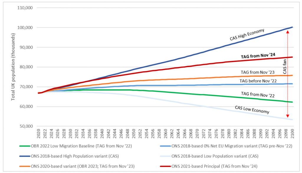
In itself, this doesn’t directly affect many appraisals: we don’t often use the population forecasts in their own right. And in any case, the discounting process dampens the importance of these long-term changes as we go further into the future. But it will filter through into higher long-term demand forecasts in the DDG, TEMPro factors and the like – often increasing scheme benefits a little.

DfT’s chart also shows how this sequence of core projections compares to the population assumptions in the ‘high economy’ and ‘low economy’ Common Analytical Scenarios (CASs). These two CAS essentially bookend the range of uncertainty in economic and demographic demand drivers.

Strikingly, the new projection starts at or just above the level used in the high economy CAS and will continue to be at or near that level into the 2030s and 2040s – which tends to be the period of maximum benefits in appraisal terms.

Of course, this CAS is not just about the population: it also assumes a higher productivity growth rate, and hence GDP per capita, than the core (and vice versa for the low economy scenario). But it does look as though this new projection is pulling the core a bit closer towards the high economy scenario.

DfT continues to see these two CASs – whose population projections are from alternative ONS scenarios and remain unchanged – as the way of addressing uncertainty about future population growth. And that’s certainly right. But I wonder whether there’s a case for re-basing them around either side of the new core population projection – perhaps as part of a full re-basing of the CAS within the next few years.

Emissions factors

The same FC notice reports on a minor update to the emissions factors for petrol, diesel and gas oil. These are the parameters for converting fuel use into greenhouse gas (GHG) emissions. DfT says these updates are minor, with diesel emissions factors about 5% lower over the long run and petrol or gas changing less than 1%. GHG emissions figures will therefore fall marginally. Electricity emissions factors are unchanged.

Optimism bias for rail opex

The guidance on rail project appraisal (unit A5.3) will be updated with ‘clarification’ on the application of optimism bias (OB) to operational costs (‘opex’ in the jargon). The brief note in the FC notice simply says that practitioners will be advised to ‘consider the importance of network-wide cost savings to the intervention in question’ when deciding whether to apply the OB uplift to gross or net opex.

Changes to wider economic impacts methods

The second FC notice focuses on a set of updates to the units covering wider economic impacts (WEIs), based on recent research and other factors. It’s a long list of mostly technical changes, some of which will affect the appraisal results for projects that include monetised WEIs (level 2 or 3 benefits). Key points include:

• The uplift factor for output change in imperfectly competitive markets (OCICM) increases from 10% to 13.4%
• Agglomeration calculations will now include public sector jobs, but will also include ramp-up periods of up to 15 years for certain agglomeration mechanisms

An updated version of the WITA software, which covers these calculations, will also be produced.

The net results of the changes will have a degree of ‘swings and roundabouts’, and individual schemes may see higher or lower benefits due to the changes.  

WEI practitioners will have to get used to some extra terminology: not only static clustering (changes in transport connectivity) and dynamic clustering (changes in land-use and employment locations), but also static and dynamic agglomeration mechanisms. The dynamic mechanisms are the ones that take time to feed through, hence the ramp-up. Just to keep us on our toes, static clustering can involve dynamic mechanisms. If you deal with the nuts and bolts of WEIs, it’s worth reading the notice over a nice cup of tea to figure it all out.

The new indicative BCR

Tucked away in the WEIs notice is news of a change in the approach to benefit-cost ratios (BCRs).

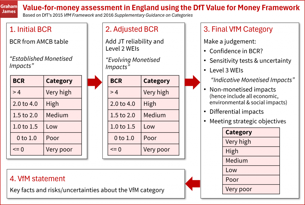
Under the current approach, as set out in DfT’s Value for Money (VfM) Framework, level 2 WEIs (also known as ‘evolving’ impacts) can be included in an ‘adjusted BCR’ but the level 3 WEIs (‘indicative impacts’) cannot. The latter can feed into a decision on the final value-for-money category, but you are not allowed to produce a level 3 BCR as such.

This seems to be changing. It’s been known for a while that DfT is updating its VfM framework. The FC notice now reveals that there will be a new ‘indicative BCR’, presumably corresponding to inclusion of the level 3 (indicative) impacts in those projects which are assessing them. We will have to wait for the updated TAG units, or the new VfM framework itself, to see exactly how it fits in to the process and how much weight it can be given.

Another option for tackling the ‘new modes’ problem

The final FC notice is about new supplementary guidance on appraising new modes: specifically, offering a new option for dealing with the TUBA ‘new modes problem’. This one’s a bit technical too.

TUBA is the software commonly used for calculating scheme benefits based on outputs from a traditional transport model such as a strategic assignment model. The problem comes up when your scheme (and hence the do-something (DS) scenario) involves a new mode of transport that doesn’t exist – or isn’t a practical option for the people involved – in the do-minimum (DM) scenario. In theory, it could also apply if a mode is taken away.

To cut a long story short, the usual way of calculating benefits can’t be done in this situation. The current solution is to create a ‘pseudo-DM’ scenario in which you pretend the new mode is there, with a ‘cost’ (journey time etc) that only attracts a tiny (but non-zero) number of users. There’s existing TUBA guidance on this if you want the full details.

The new guidance, now released in draft, is based on recent research and focuses on new rail lines or stations. It sets out another solution to the problem. This is based on what the new mode’s users did in the DM, and hence the cost difference between their previous mode in the DM and their use of the new mode in the DS.

The guidance describes both methods: the existing ‘own-cost’ approach and the new ‘alternative mode’ approach. It sets out their pros and cons, and when each one might be suitable. There is an accompanying spreadsheet of worked-example calculations.

This new guidance is due due to go live in May 2025. TUBA itself won’t need updating for this. DfT says there may be minor drafting or technical changes when it goes live, but the basic principles won’t change from the draft version.

Contains public sector information licensed under the Open Government Licence v3.0

Share this: