 by
by Graham explains the key points in the latest round of TAG updates – and what they could mean in practice
This post was originally written in early November 2023 when these updates were Forthcoming Changes. It has been updated in December 2023 to reflect the ‘live’ changes.
The DfT has published the latest round of updates to its Transport Analysis Guidance (TAG). These were announced in October as Forthcoming Changes, and have now gone live with publication of (most of) the actual updated TAG units, databook and other items.
The updates include :
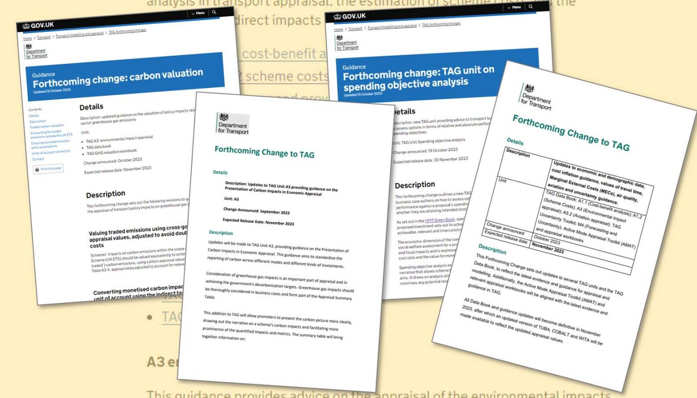
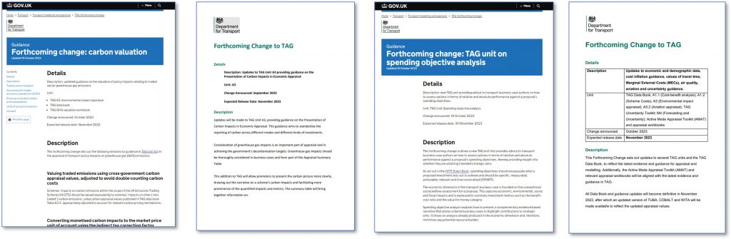
- Valuation and presentation of carbon impacts
- New guidance on spending objective analysis
- … and a range of other updates
I’ve updated my Tag-at-a-Glance page to give a unit-by-unit (or workbook-by-workbook) summary of these changes. So in this post, I’ll just cover the highlights and some of the background to them.
Attendees at the recent TAG Conference heard about a bumper set of modelling guidance updates. These are not part of the current round, but are expected to come out by the end of the year as forthcoming changes and to go live in May 2024.
Changes to carbon valuation and presentation
There are important changes to both how carbon is valued for appraisal purposes, and how carbon impacts should be presented.
Embodied carbon in construction materials, such as concrete and steel, will now be valued as a carbon impact in appraisals. Until now, this impact has been treated as covered by the carbon prices that manufacturers pay under the UK or EU emissions trading schemes, and therefore appears under the ‘cost’ side of the BCR. Theoretically neat, but means it gets a bit hidden. In future, it will be valued explicitly, in the same way as non-traded emissions (such as tailpipe emissions), on the ‘benefits’ side of the equation. Obviously a carbon increase will be a negative number (disbenefit) and vice versa. To avoid double-counting, this value will be net of the trading-scheme carbon price, so we will need to not only estimate the embodied carbon impact (which we should be doing anyway) but also get familiar with using carbon-price forecasts.
Carbon valuations should be converted from factor costs to market prices. If you’re not familiar with this terminology, don’t worry. It’s just a technical adjustment to do with VAT, and your appraisal team will do it for you. It will increase the value of all carbon impacts (positive or negative) by 19%.
The new Carbon Summary Table brings all the carbon information together in one place. Under current practice, it’s not always easy to get a complete picture of the carbon impacts when reading an appraisal report or business case. This new table should really help. Think of it as like the Appraisal Summary Table (AST), but focusing on the carbon impacts. The template is online. The guidance confirms that the reporting should be proportionate to the business case stage and the availability of appraisal outputs. So it shouldn’t need any information that we wouldn’t already have: for example, at SOBC stage, we might only be able to complete the qualitative elements.
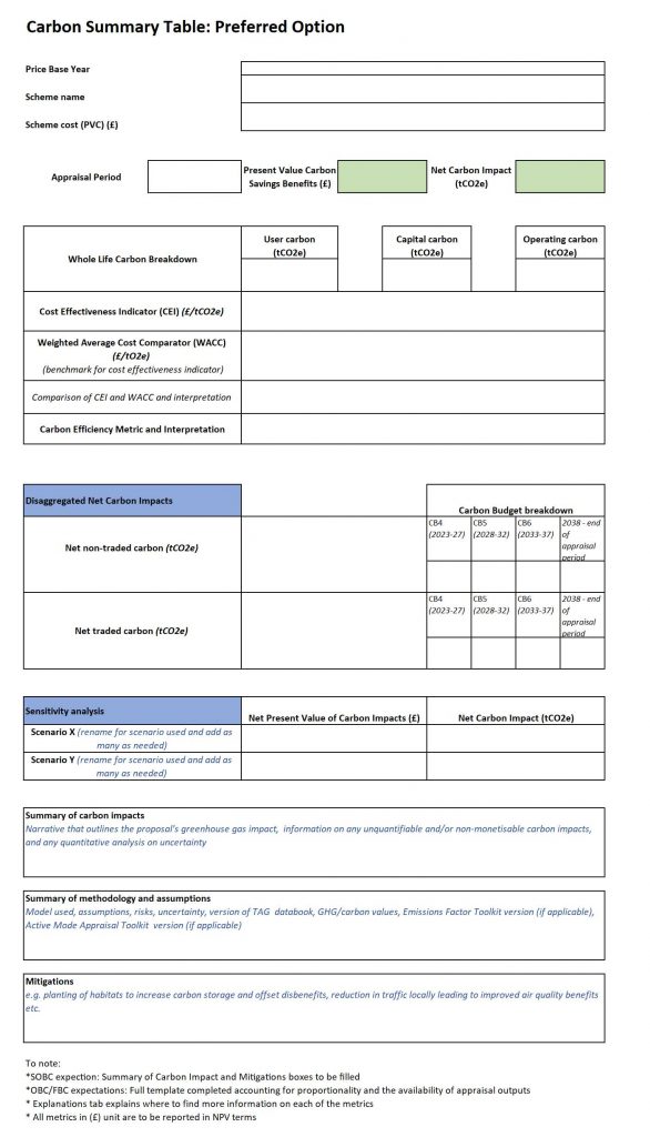
The Carbon Summary Table also introduces three new carbon reporting metrics. These again use existing appraisal results. They aim to summarise the carbon impacts and show the potential trade-offs in decision-making. For example, the “cost-effectiveness indicator” is the net non-carbon impact per tonne of CO2e saved or emitted, and is intended as a guide to which interventions save or emit carbon in a relatively more/less valuable way for society.
New guidance on spending objective analysis
This is all about tying the appraisal results (in the economic case) back to the scheme objectives (in the strategic case) to show how well the scheme or the different options actually meet those objectives. The 2020 Green Book Review highlighted that this doesn’t always happen: there can be a disconnect between the strategic and economic cases, with objectives focused on one set of things but appraisal focused on another. Transport schemes are not immune from this, and although a good business case will already tie the two together, this new guidance will hopefully support wider adoption of this best practice.
The basic principle is that ‘spending objective analysis’ is an evidence-based narrative, highlighting a proposal’s contributions to strategic aims. It complements, and should be considered alongside, the traditional economic aspects. Importantly, it draws on the economic case results (including things that do or don’t feed into the BCR) – it’s not a new set of analysis.
The new guidance covers spending objective analysis at the long-list and short-list stages, and how it should also inform project evaluation.
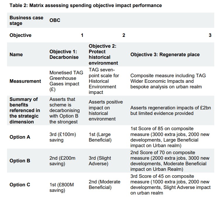
The key new concept is the Spending Objective Analysis Statement (SOAS). This is a narrative summary (based on the appraisal evidence) of the impacts on the scheme objectives, and any trade-offs between options.
The SOAS starts with an initial presentation of those impacts, including each option’s absolute performance and ranking their relative performance. The guidance recommends presenting this in a table, and gives an example. Back in the Autumn, at the TAG Conference, this table had been described as the Spending Objective Analysis Summary Table. This terminology isn’t used in the guidance, perhaps because the table is just a recommendation rather than a requirement. It’s a good recommendation, though, and I still expect we’ll call it the ‘SOAS table’. Cleverly, the recommended table format includes a line to refer-back to the benefits stated in the strategic dimension: another way to check that the strategic and economic cases are aligned.
The next part of the SOAS is to assess the key uncertainties, to understand how they might affect the relative and absolute performance of options. This could cover a wide range of uncertainties (anything from the national economic picture to uncertainties in the modelling process) but is really about focusing on the most important ones and signposting to the evidence presented elsewhere in the appraisal.
The SOAS finishes by drawing these aspects together into an evidence-based narrative summary of the options’ impacts on the spending objectives. It should set out any trade-offs (as different options might be best for different objectives). It could also include an overall ranking of options based on some form of decision-rule, but this is not required.
DfT sees the SOAS as being proportionate and succinct, similar to the Value for Money Statement. It should signpost to the detailed evidence rather than re-stating it. Around two pages is seen as the rule-of-thumb.
New numbers and other general updates
The last set of updates covers a lot of ground in updating the TAG Data Book, several units and some of the supporting spreadsheets, tools and software. I’ll only cover some highlights here.
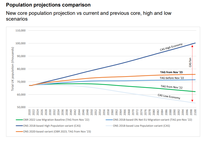
The headline item is an update to the economic and population forecasts: things like GDP per capita, which feeds into future values of time and hence into the benefits of many schemes. TAG uses forecasts from the Office for Budgetary Responsibility (OBR) and this update reflects the latest. As well as the Data Book, the new values feed into the appraisal worksheets and the Active Mode Appraisal Toolkit (AMAT) – which have therefore all been updated too. Updated TUBA, COBALT and WITA files are also due out shortly.
This update includes a change in population projection. Although a significant change, the notice has a handy chart which confirms it’s not a radical departure from the range of population forecasts that have been used over the last few years. The other key point to remember is that the discounting process dampens the importance of such long-term changes as we go further into the future.
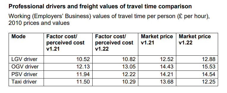
Also being updated are the values of time for professional and freight drivers, some of the values for marginal external costs (MECs), and some of the parameters used in the AMAT.
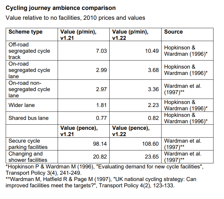
One of the latter is the set of cycling journey ambience values – the ‘pence per minute’ benefits from upgrading the infrastructure quality of a cycle route. Most of these are increasing a little but there’s a big jump in the ‘off-road segregated cycle track’ value which goes up from roughly 7p to 10p per minute. I’ve updated my ready-reference chart accordingly.
These values are, of course, relative to the existing facilities. On schemes that are upgrading infrastructure from little or no provision to segregated provision, this can be quite a valuable increase in benefits. Where the infrastructure upgrade is only modest, it may be less so. On some schemes the ambience benefits are dwarfed by the health benefits for new users – which are also increasing with this update (by around 10-20% when I ran some tests).
Away from the numbers, there’s an update to the Uncertainty Toolkit guidance on the scenarios (particularly the Common Analytical Scenarios) to consider in different situations. My impression is of a slight general ‘bumping-up’ of what is required. This includes the need for a qualitative discussion of how different CAS could affect the scheme or the options, even when some CAS are being run quantitatively.
To round off the changes, there are miscellaneous updates to other areas of TAG. These include real cost inflation (unit A1.2 section 3.6), air quality appraisal when a scheme may lead to exceedances (A3), and greenhouse gases in aviation schemes (A5.2). Finally, back in September Tempro 8.1 was released which reinstated the ability to generate local traffic growth factors, and this is reflected in unit M4.
What does it all mean?
A lot of these changes are, as is often the case, relatively routine incremental updates. Appraisal practitioners will be familiar with incorporating them in standard processes, new appraisals, and (when proportionate) ongoing existing ones.
For me, the most significant ones are the carbon appraisal changes and the new unit on spending objectives analysis. Explicit valuation of traded carbon fills an important gap in the practical visibility of a scheme’s carbon impacts: the tailpipe emissions figure is usually explicit in appraisals but the embodied carbon impact is (until now) rarely so. The carbon summary table is also welcome as a way of bringing the whole carbon picture together. Together, these carbon valuation and presentation changes are important and welcome.
The new guidance on spending objectives analysis might look at first glance like a new requirement, but it’s really about best-practice in tying the appraisal results back to the objectives. It’s a further incremental step in the ongoing process of bringing spending objectives – and the question of ‘is this scheme delivering what we originally wanted?’ – closer to the heart of appraisal and decision-making. Hopefully it will help to bring more business cases up to best-practice standards in this respect.
Let me know (in a comment below, or on my social media channels) what you make of these changes, and if you think I should do a more detailed post to delve into any of them.
Extracts from TAG are public sector information licensed under the Open Government Licence v3.0.